


Last Updated: August 2026
A Monte Carlo simulation valuation runs a value thousands of times. Each unsure input is drawn at random from a set range. So the result is a spread of business values, not one number. Most jobs run 10,000 runs or more before the output settles into a clear picture. When one estimate cannot capture the real risk in a deal, Sofer Advisors uses it to show the whole range.
The method earns its place when a deal hinges on events that have not yet happened. Earnouts, contingent payments, and option-like terms all shift with future results, so a single figure hides the true spread of risk. By pricing thousands of paths at once, the model shows both the expected value and the odds of each outcome around it. That is why it fits complex deals a fixed model cannot.
Key Takeaways
- A range, not a point: It models thousands of outcomes and returns a spread of values, not one fixed figure.
- Built for the unknown: It fits earnouts, contingent consideration, option-like payoffs, and early-stage firms where outcomes vary widely.
- Inputs drive it all: Each input is set as a range with a shape. The result is only as good as the guesses behind it.
- Kin to sensitivity analysis: It moves all inputs at once. Sensitivity analysis moves one at a time, and scenario analysis tests a few fixed cases.
- Standards still apply: It supports fair value work under ASC 805 and ASC 820, yet each input must be documented and held up under USPAP.
These points frame when the model earns its added cost. The sections below show how it works, what it needs, and where its limits lie.
What is a Monte Carlo simulation valuation?
A Monte Carlo simulation valuation is a model that runs a calculation thousands of times. Each time, it draws every unsure input at random from a set range. Then it maps the full span of values. A single-point model, like a standard discounted cash flow (DCF) analysis, fixes each input. It returns one enterprise value. The model swaps those fixed points for ranges. So revenue growth, operating margins, and the discount rate each become a range, not a guess.
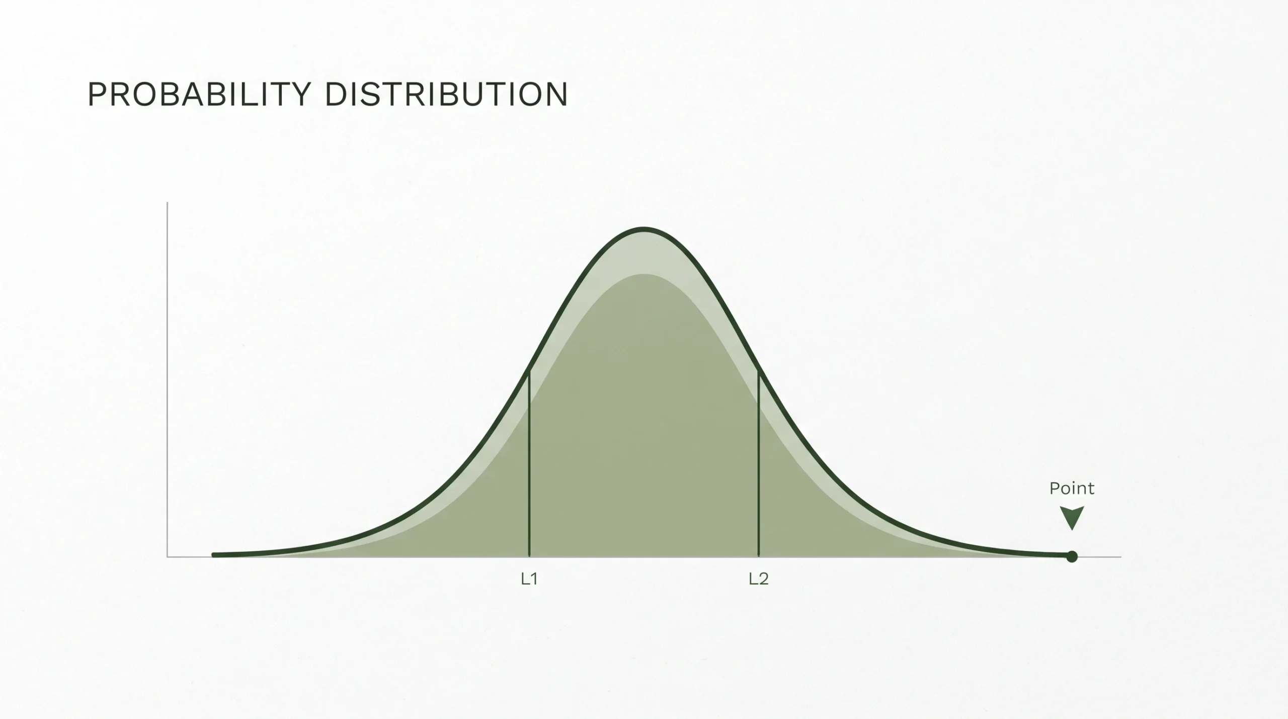
After thousands of runs, the results form a spread. It shows the likely value at the center and the range of outcomes around it. Two firms can share the same average value yet carry different risks. Only a range makes that gap clear.
When should a valuation use simulation?
Use it when an asset carries high risk and depends on several linked inputs. The clearest cases have payoffs that are path-dependent or option-like. Here the result shifts sharply based on how future events unfold. Earnouts, contingent consideration, complex stock options, and early-stage firms with shaky cash flows all fit. When outcomes vary widely, one number hides more than it shows.
Contingent consideration inside a purchase price allocation is a common trigger. When a deal includes an earnout, the value of those payments rests on set targets. Those targets may or may not be met. The model prices every payout path against set odds. For a stable, mature firm, a single-point income approach is enough. The method should match the risk in the asset.
How does the simulation process work?
It works in three steps: build a model, set each input as a range, then run it thousands of times. An analyst first picks the output, such as total equity value. Next they name the drivers that shape it. Those drivers often include revenue growth, EBITDA margins, capital spending, the terminal growth rate, and the weighted average cost of capital. Each one gets a range, not a fixed figure.
Software then runs thousands of random passes. In each pass, the model draws one value from every input range and records the result. Once the runs end, the results form a spread. It is often shown as a histogram, which displays how often each value came up. From it, an analyst reads the likely value at the center and the tail risks at the edges.
What inputs and assumptions drive the model?
The main inputs are revenue growth, EBITDA margins, capital spending, a terminal growth rate, and the weighted average cost of capital. An analyst sets a base case for each one. They use past results, industry forecasts, and the firm’s risk profile.
Each input then gets a range to reflect real risk. Rather than a single mean, an input is set by a span, a spread, and a shape. Revenue growth might follow a normal curve. It clusters most outcomes near a central value while allowing drift on either side. Links between inputs matter too, since related inputs should move together. The team sets these ranges from market data such as the Kroll Cost of Capital Navigator. So each run reflects the real risk in the business, not a handy guess.
How does it differ from sensitivity analysis?
Monte Carlo simulation, sensitivity analysis, and scenario analysis all test how inputs affect value. But they work in different ways. Sensitivity analysis moves one input at a time to show which drivers matter most. Scenario analysis groups a few inputs into fixed cases, such as best, base, and worst. Simulation moves all inputs at once across thousands of runs. So it can gauge the odds of combined outcomes, not isolated ones.
| Method | How inputs move | What it produces | Best used for |
|---|---|---|---|
| Single-point DCF | Fixed values | One enterprise value | Stable, predictable earnings |
| Sensitivity analysis | One at a time | Impact of each driver | Finding the key variables |
| Scenario analysis | A few fixed cases | Two or three outcomes | Framing a range of futures |
| Monte Carlo simulation | All at once, random | A probability distribution | Wide, path-dependent risk |
These methods pair well in practice. Sensitivity analysis points to the inputs that deserve the most study. Simulation then models those inputs together to reveal the odds of each combined result. A single-point DCF still supplies the cash flow logic the model runs on top of. Used in order, they show an owner which drivers matter. They also show how much total risk sits in the value.
What are the limits of this method?
The method has real limits. The biggest is that the output rests fully on the inputs it is fed. So poor or biased guesses yield a result that looks precise but means little. The math runs cleanly on flawed data and still returns a tidy spread, which breeds false trust.
Cost and effort are the other limits. It needs special software, careful setup, and skilled review. So it is best saved for cases where the risk earns the extra work. For simpler jobs, a standard income approach is faster and just as sound. The Appraisal Foundation, which maintains USPAP, ties the trust in any model to the support behind its inputs. So care in each guess matters more than the tool itself.
How does Sofer Advisors approach simulation?
Sofer Advisors treats it as one tool within a wider process, chosen only when the asset calls for it. Large firms such as Kroll and Alvarez and Marsal often run high-volume portfolio work on standard systems. Solo practitioners may lack the depth to set up a model well. The firm sits between the two. It brings senior-level rigor to middle-market owners, with a full W2 team of 14 and subscriptions to all major valuation databases.
The work follows The Sofer Difference, a four-phase process of Discovery, Diligence, Analysis, and Delivery. It keeps every input documented and easy to trace. That matters most when a model must survive scrutiny from auditors, the IRS, or opposing counsel. Guided by the Heart of a Teacher, David Hern CPA ABV ASA and the team walk owners through the logic of each input, not just the final range. The firm has earned 180+ five-star Google reviews and Inc. 5000 recognition in 2024 and 2025.
Frequently Asked Questions
What is the difference between a Monte Carlo simulation and a DCF analysis?
A discounted cash flow (DCF) analysis is a fixed model that gives one enterprise value from a set of projections. It treats every input as fixed. A Monte Carlo simulation swaps those inputs for ranges. It runs the math thousands of times, giving a span of values instead of one. The two work together. The model often uses DCF logic to build each run, then adds a view of the risk around the result.
Is a Monte Carlo simulation the same as sensitivity analysis?
No. Sensitivity analysis moves one input at a time. It gauges how much each driver shifts the value and flags the guesses that matter most. A Monte Carlo simulation moves all inputs at once across thousands of runs and reports the odds of combined outcomes. Sensitivity analysis tests single drivers in isolation, while the model captures how those drivers interact. The team often uses both: one to find the key inputs, the other to model overall risk.
How many iterations are needed for a reliable simulation?
It depends on how complex the input ranges are, not on a fixed count. Most valuations run 10,000 to 100,000 iterations to reach a stable result. A higher count helps tail risks and extreme outcomes show up well in the final spread. Too few runs add numerical noise that can blur the true shape of the result. An analyst raises the count until the output settles and stops shifting much between runs.
What software is used for Monte Carlo simulations in valuation?
Analysts rely on pro tools such as @RISK and Crystal Ball, or on custom models built in Python or R. These tools let an analyst set links between inputs and build high-resolution output spreads across many runs. Standard spreadsheet formulas often lack the power for tens of thousands of runs. The firm works in proven technical setups to keep every model accurate and easy to reproduce for tax and financial reporting.
Is a Monte Carlo simulation required for ASC 805 purchase price allocations?
No standard flatly requires it. But it is often the best fit for path-dependent instruments and contingent consideration under ASC 805. When deal terms include layered earnouts or multi-tier targets, fixed models usually fail to capture the real risk. Because financial reporting needs a fair value estimate, an analyst must pick the tool that fits the instrument. The team uses it when it yields the most accurate and defensible fair value.
How do you defend a Monte Carlo valuation in court?
You defend it by documenting the basis for every input and showing why the chosen ranges reflect real market conditions. An expert witness must show that the guesses were picked to capture true risk, not to steer the result toward a set number. Clear records of the model and each input are key for testimony. The Sofer Advisors team has given expert witness testimony in 11+ cases across Georgia, Florida, California, and New Mexico.
How does the model handle correlations between input variables?
The model uses covariance matrices or copulas so that related inputs move in a real relationship. Revenue growth and operating costs, for example, should not drift apart in ways that never happen in real life. If an analyst skips these ties, the model can yield odd results, such as high revenue paired with low costs. Sound correlation modeling keeps the combined outcomes credible.
How much does a business valuation from Sofer Advisors cost?
Standard business valuation services run from 7,500 to 25,000 dollars. The price depends on how complex your finances are and the purpose. Simpler jobs for planning or tax fall toward the low end. Deals, financial reporting, and litigation support that need simulation and deeper work fall higher. Contact Sofer Advisors for a fee quote matched to your situation and the level of modeling your engagement calls for.
Related Case Studies
- What Is a DCF Valuation? Complete Guide to DCF Method
- What Are the Discounted Cash Flow Techniques? A Guide
- Terminal Value Formula: How to Calculate It in a DCF
Executive Summary
A Monte Carlo simulation valuation runs thousands of runs across ranges for unsure inputs. It gives a span of values rather than one figure. It earns its added cost when an asset carries wide, path-dependent risk, such as earnouts, contingent consideration, or early-stage cash flows. Most jobs run 10,000 runs or more to reach a stable result. Because the output is only as sound as its inputs, every guess must be documented and held up under ASC 805, ASC 820, and USPAP.
What Should You Do Next?
Start by checking whether your asset needs it. A stable firm with steady earnings is served well by a standard income approach. If earnouts, options, or wide risk are in play, gather at least three years of financials, management forecasts, and industry data. That way the input ranges reflect real risk. Then flag the few inputs that carry the most weight in your outcome.
For a model you can defend, work with David Hern CPA ABV ASA, whose team designs and defends these valuations for financial reporting, tax, and litigation. Schedule a consultation to discuss whether this approach fits your situation.
People Also Read
About the Author
This guide was prepared by David Hern CPA ABV ASA, founder of Sofer Advisors, a business valuation firm headquartered in Atlanta, GA serving clients across the United States. David holds dual accreditations as an Accredited Senior Appraiser (ASA) and is Accredited in Business Valuation (ABV), credentials recognized by the IRS, SEC, and FINRA. He also holds the Certified Exit Planning Advisor (CEPA) designation. With 15+ years of valuation experience, David has served as an expert witness in 11+ cases across multiple jurisdictions and built Sofer Advisors into an Inc. 5000-recognized firm with 180+ five-star Google reviews. Its full W2 employee team maintains subscriptions to all major valuation databases and operates under a next business day response policy. For professional business valuation services, contact Sofer Advisors at soferadvisors.com/contact-us/.
Disclaimer: This content is for informational purposes only and does not constitute professional valuation advice. Business valuation conclusions depend on specific facts and circumstances. Contact Sofer Advisors for guidance regarding your specific situation.